So, this is the fourth day of data science, I don't know if I can explain it well, but yes at the moment I just finished building a salary generation app for data scientists and other posts.

I will walk you through the steps I followed.

Step 1: Loading the CSV dataset you can get this from a website called Kaggle.

Step2: Check for null and duplicate values and remove the same if they exist, in my case they didn't this time

Step 3: I did describe and see how the mean and max values are related. In this case

they were so high and so close, so I thought there were outliers

Step 4: Identifying the outliers and handling them.

df_2 = df['Salary in USD']
ax = sns.boxplot(data=df_2, orient="h", palette="Set2")

Above the code which gives you a block and you can see the outliers both in the max and min zone.

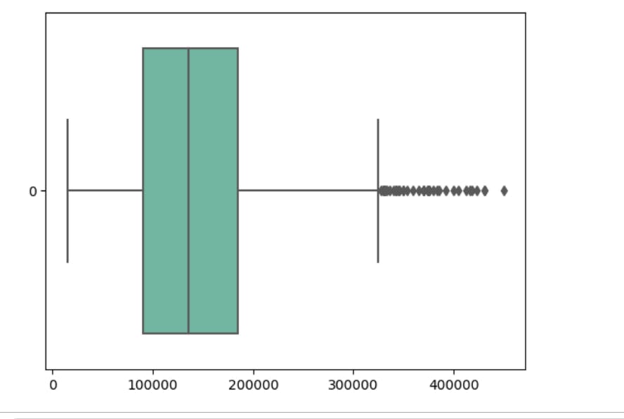
You can see how much are the outliers.

The next step is to normalize the data and impute the outliers.

There are several ways you can handle outliers but I did replace the outliers with the median values for achieving normalized distribution. You can check other ways on the internet.

Next, I was kind of skeptical that the pictures are reliable, so I decide to confirm the same with the help of scripts.

Below is the script, you can have it executed for different columns.

outliers = []
def detect_outliers_zscore(data):
    thres = 3
    mean = np.mean(data)
    std = np.std(data)
    # print(mean, std)
    for i in data:
        z_score = (i-mean)/std
        if (np.abs(z_score) > thres):
            outliers.append(i)
    return outliers# Driver code
sample_outliers = detect_outliers_zscore(df['Year'])
print("Outliers from Z-scores method: ", sample_outliers)

This is the z-score method, which is a cool topic in statistics but currently out of the scope of this post.

df['Salary in USD'] = df['Salary in USD'].fillna(df['Salary in USD'].median())

Used this expression to replace all the above outliers with the median value. We can check this by plotting the box plot again to see the outliers are gone.

Step 5: Next, you can do a couple of plots to analyze the data.

Below is the code for the same.

import matplotlib.pyplot as plt
for col in ['Salary', 'Salary in USD', 'Year']:
    print(col)
    print('Skew :', round(df[col].skew(), 2))
    plt.figure(figsize = (15, 4))
    plt.subplot(1, 2, 1)
    df[col].hist(grid=False)
    plt.ylabel('count')
    plt.subplot(1, 2, 2)
    sns.boxplot(x=df[col])
    plt.show()

Bar plots are great for analyzing categorical data so having handled all the numerical data, we can move ahead to do categorical data.

cat_cols=df.select_dtypes(include=['object']).columns
num_cols = df.select_dtypes(include=np.number).columns.tolist()
print("Categorical Variables:")
print(cat_cols)
print("Numerical Variables:")
print(num_cols)

con = np.concatenate((cat_cols, num_cols))
print(con)

for col in con:
    plt.figure(figsize=(15,7))
    sns.barplot(x = df[col],y = df['Salary'])
    plt.xticks(rotation = 'vertical')
    plt.show()

This is the multivariate analysis where you will see the relation between the independent variable - the salary price in USD in this case with the other features.

Univariate analysis is another way to analyze numerical data you can do the frequency count for the variables to see the value counts.

Python provides a function to do this as well.

Step 6: This is the step where you see the correlation of various numerical variables. To do this more effectively, there is another sub-step we have to follow is to handle the categorical data. There are many ways to handle categorical, what I found more effective in this case is the use of label encoding.

mapping_dictionary_value={'Expert':1,'Intermediate':2,'Director':3,'Junior':4}
df['expertise_level_ordinal']=df['Expertise Level'].map(mapping_dictionary_value)
df

This code will create a new column and map the categorical variables to the values specified in the dictionary. You can first decide which are the ordinal data and achieve the normalization of the data using this method. It is very easy as well.

df.drop(['Employment Type'], axis=1, inplace=True)
df.drop(['Experience Level'], axis=1, inplace=True)
df.drop(['Expertise Level'], axis=1, inplace=True)

Remember to remove the main columns from the data frame to make the table look pretty.

Step 7: Next in some cases you may come across categorical data which are nominal and huge in number if you value count the column.

df['Salary Currency'].value_counts()

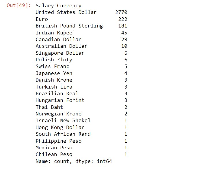
This was the result.

So in this case you can do conditional labelling based on the central tendency of the value count

So based on the counts, I decide to the following:

def setcategory(text):

    if text == 'United States Dollar' or text == 'Euro' or text == 'British Pound Sterling':
        return 1

    elif text == 'Indian Rupee' or text == 'Canadian Dollar':
        return 2

    else:
        return 0


df['Currency_value'] = df['Salary Currency'].apply(lambda x: setcategory(x))

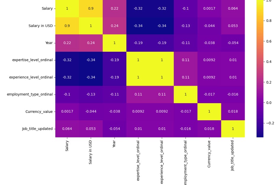
Now the heat map looks like this. Pretty neat right?

Model Building

The first step of model building is to decide on the train and test data.

test = np.log(df['Salary'])
train = df.drop(['Salary'],axis = 1)
X_train, X_test, y_train, y_test = train_test_split(train,test,
                                                   test_size=0.15,random_state=2)
X_train.shape,X_test.shape

Salary which is the main variable we are interested in is the test data and everything else is the trained data.

Then we split the train and test data with the above.

# we will apply one hot encoding on the columns 
# the remainder we keep as passthrough i.e no other col must get effected
# except the ones undergoing the transformation!

step1 = ColumnTransformer(transformers=[
    ('col_tnf', OneHotEncoder(sparse_output=False, drop='first',handle_unknown = "ignore"), [1])
], remainder='passthrough')

step2 = LinearRegression()


pipe = Pipeline(steps=[('step1', step1),
                       ('step2', step2)])
pipe.fit(X_train, y_train)

y_pred = pipe.predict(X_test)

print('R2 score',metrics.r2_score(y_test,y_pred))
print('MAE',metrics.mean_absolute_error(y_test,y_pred))

We are applying columnTranformer to the linear regression to create the pipe and then fit the x and y train data to predict the results with X test data.

I hope this post helps you to visualize the entire process.